
After an adjustment, it is tempting to look for a nicer-looking surface and call the job done. A useful comparison asks a more precise question: what changed in the measurements, under conditions that were otherwise comparable?
Write down the conditions
Keep the same build surface, sampled area, grid, bed temperature, and probing setup where possible. Give the printer a similar settling period before each run. Note the specific change you made rather than bundling several adjustments into one comparison.
Use the optional Measurement context beside each input to record the temperature, surface, setup, date, and notes. The comparison calls out missing or different declared conditions without claiming that matching text proves matching physical conditions. Keep the original console output as well. The extra context is often more useful than another decimal place.
Make the charts comparable
Enable matching scales and choose the same height reference in both panels. A fitted scale can make subtle variation fill the chart, which is helpful for inspection but can distort a visual comparison between runs.
Use measured heights to inspect original offsets, centre on mean to compare variation around each average, or remove fitted tilt to inspect the remaining shape. Each setting answers a different question. Choose it deliberately and use it consistently.
Look beyond one number
Check the original range and standard deviation, then inspect fitted rise and residual variation. A changed mean with a similar spread can reflect a changed reference. A smaller range on a coarser grid can reflect a missed local feature. Neither observation is enough on its own to diagnose an improvement.
The heatmap and measured-values table help you locate differences. When a result looks promising, another run under the same conditions can show whether it repeats. A measurement that repeats is more useful than a single attractive chart.
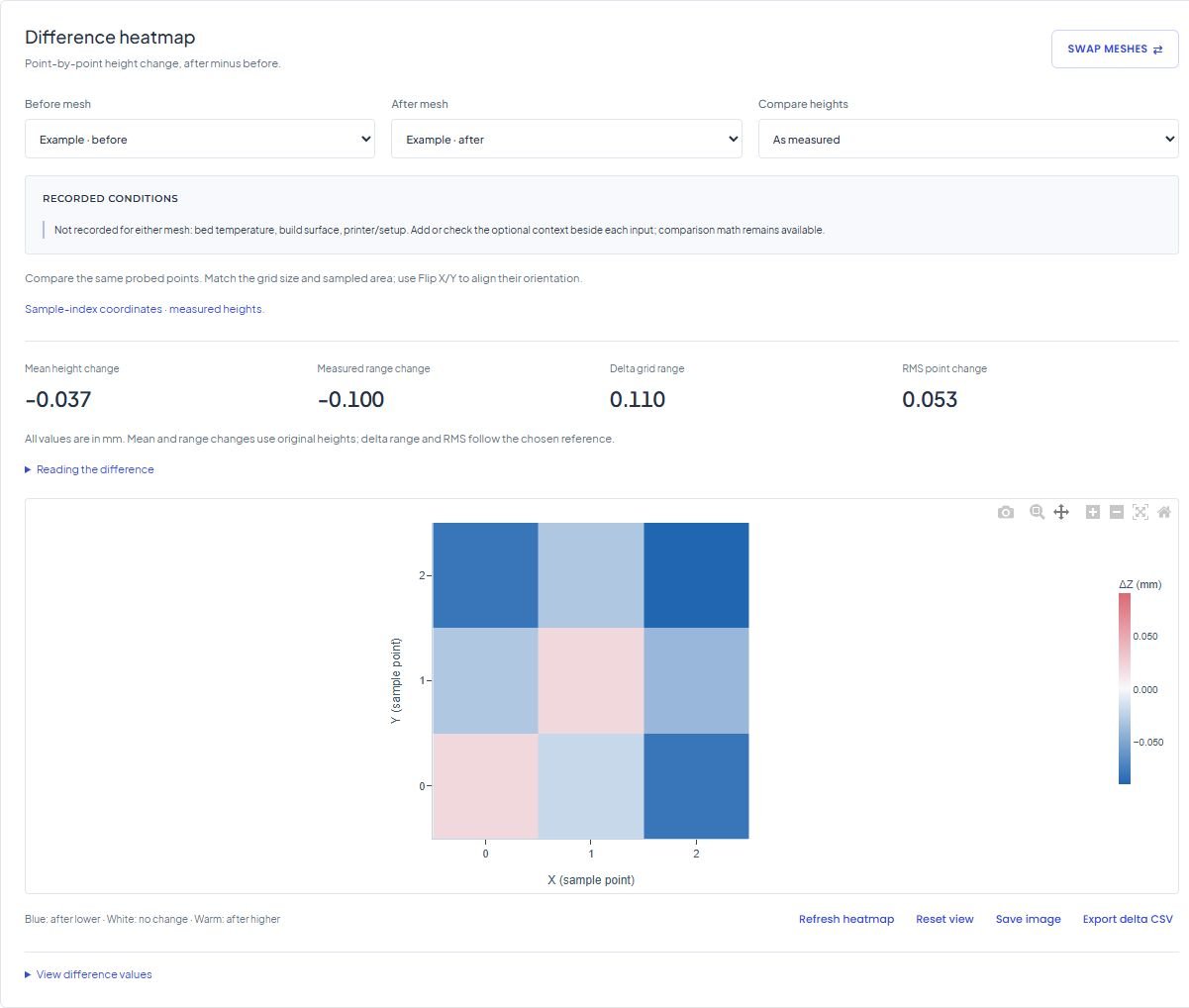
For a point-by-point view, choose a before mesh and an after mesh in Difference heatmap. Blue means the after point is lower; warm colours mean it is higher. The chart uses a symmetric scale around zero. Matching the grid and sampled area is required, and you still need to check the probing origin and orientation yourself.
Keep the evidence together
Export the original CSVs and save the workspace with its display settings. Chart images are useful for sharing an observation; the numeric source lets someone check it. A browser workspace is convenient, while an exported file gives you a separate record.
For a step-by-step reference, see comparing two mesh runs.